The Magdalen Islands (Îles-de-la-Madeleine) are an archipelago located in the center of the Gulf of Saint Lawrence (Eastern Canada). The heart of the archipelago is made up of seven rocky islands connected by long sand barriers, sand spits, dunes, and salt marshes. Including internal lagoons, the islands cover about 330 square km. The archipelago is sparsely populated and counts about 12K permanent inhabitants.

In June 2023, OSM describes the islands’ coastline, road network, some trails as well as some human and natural features. Overall, the islands were mapped using about 56K nodes, 5K ways, and 116 relations (Figure 1).

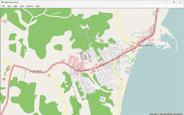Figure 1: Cap-aux-Meules, before starting the project—Historical OSM data as of June 30, 2023, on Maperitive.

It was after traveling to the Magdalen Islands on vacation that I set out to update the OSM map. Upon my return, and over a 9-month period, I edited the existing OSM content, correcting geometries and adding as many features as I could, using local knowledge and available images (Figure 2).

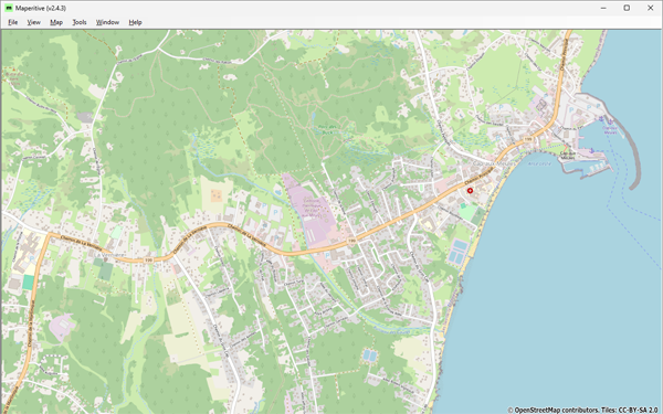Figure 2: Cap-aux-Meules, at the end of the project—OSM data as of February 28, 2024, on Maperitive.

Once completed, I had increased the number of nodes and ways by 10 folds, the number of relations by 30. All this did not happen without a lot of work, questions, and sometimes big surprises! Here is a summary of what I did.

Fieldwork Prior to Image interpretation

We were several friends visiting the islands together. Everyone knew I was collecting data for mapping in OSM and, as usual, some were teasing me when I was moving around tagging features with a GPS! With their help, I was able to bring together a wide range of islands’ landscapes from photos and videos we all took during our stay (Figure 3). In addition to photos, videos, and GPS tracks, I also accumulated receipts for my purchases, which gave me the names and addresses of some businesses and stores I visited.

Figure 3: View of the Cap-aux-Meules Nautical Club from a nearby observation point.

During my stay, I paid attention to landscapes I was unfamiliar with, particularly sand dunes and vegetation (Figure 4). I also had a look at buildings and their distribution outside the urban environment. On the other hand, the coastline and associated infrastructure did not pose any interpretation problem as I am familiar with coastal environments. In this context, the islands tide magnitude (about a meter) just simplified the delimitation of the coastline at MHWL.

Figure 4: Informal hiking trail toward L’Étang-du-Nord (Îles-de-la-Madeleine) showing islands’ typical vegetation.

GPS Tracks and Images Adjustment

In addition to GPS tracks from OpenStreetMap, I used those from Strava Global Heatmap (SGH). This was a great discovery! SGH is an image of Strava users GPS tracks density that can be used with OSM. The number of users (e.g., cyclists, runners) who traveled the islands is so large that it allowed me to adjust the geometry of most of the road network and main hiking trails. SGH is available in JOSM via a plugin for Chrome and Firefox browsers. However, aligning satellite images with the SGH can be difficult when it obstructs the road network visibility (Figure 5). To overcome the problem, I first adjusted the road network and main hiking trails on the SGH, then aligned the images to those roads/trails. This alignment was particularly useful in areas with rolling topography.

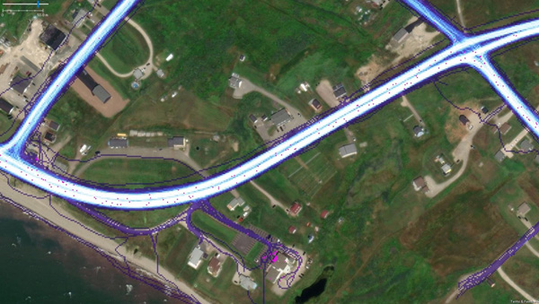Figure 5: Overlay of Strava Global Heatmap (SGH) and GPS tracks from OSM (pink dots) on Esri World imagery (Havre-aux-Maisons, Îles-de-la-Madeleine).

Available Satellite Images

All available images are generally well georeferenced. However, except for Sentinel-2, I could not find details on the orthorectification process or what type of digital elevation model was used, if any. Without using it (i.e., DEM or DSM) the images are distorted where there are changes in ground elevation and the effect increases with the viewing angle. Each following image was used, according to its characteristics.

Esri World Imagery: The primary image used. The most recent one except for the eastern end of the islands. Probably taken after the storms of 2019 or Hurricane Fiona in 2022. The viewing angle is not negligible, causing distortions on buildings and around cliffs.

Mapbox Satellite: An almost vertical image that shows little distortion. The image is clear but older than that of Esri World.

Bing Aerial Imagery: The image seems older than the other ones but is of better quality for the western part of the islands. Unfortunately, its resolution over the eastern end made it useless.

Sentinel-2: I used a Sentinel-2 image from summer 2023 as a validation data source. Its resolution is low, but it allowed me to locate some large recent features seen in the field.

Mapping Process

I chose to carry out my project using JOSM. I’ve been using the software for a while, which offers several tools that I consider essential.

Keeping Track of Mapped Areas

For mapping projects of this scale, I keep track of which areas have been mapped as well as the one in progress in a dedicated .osm file. Both areas are delineated using different tags (Figure 6). In order to prevent accidental uploads, I add the attribute upload=never to the header.

Where possible, the working area is small and its boundary easily visible on the ground (e.g., roads). When completed, the current working area is joined to the mapped area polygon, and the next working area is delineated.

Figure 6: The map production tracking layer, with mapped area (white) and current working area (yellow).

Iterative Data Capture Operations

I generally use the same sequence of operations to map all the features I’m interested in. My main interest is to “put colors on the map”, but my priority is to fit the images on available GPS track when required. To make both easier, I divide my edits into the following steps:

1. Download OSM data for a working area.
2. Align images to available GPS tracks.
3. Map a subset of features on a temporary layer.
4. Merge the layer with OSM data once completed.
5. Run the Validator to detect and fix errors.
6. Upload the data to OSM.
7. Back to step three unless everything is mapped!

Some of above steps need further explanations. In step 1, The OSM data layer is saved as a file since a working area can take several days to complete. In step 2, aligning images using Strava Global Heatmap required first adjusting the geometry of the existing transportation network to the SGH (Figure 5), and then aligning each image to the network. In Step 3, dividing map features into thematic subsets made it easier to track which features are mapped and which need to be mapped (see next section). When an existing feature needs an update, it may be easier to capture it again on the current layer and merge them later. In step 5, among the errors will appear as duplicate or overlapping features those that were capture again for an update. I strongly suggest to use the ReplaceGeometry tool to do this (Figure 7). It allows us to replace the previous geometry with the new one, while retaining tags, feature history, and nodes. It is a way to acknowledge the work done by the previous contributors.

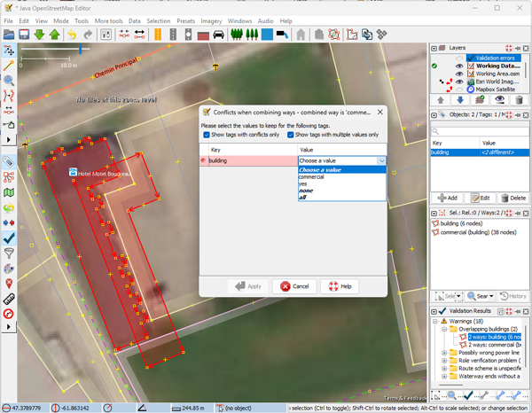Figure 7: Replacing an existing feature with the new version using the ReplaceGeometry tool.

Hierarchy in Mapped Features

The diversity of OSM’s content reflects the diversity of interests of its contributors. Since mine is to “put colors on the map”, it implies a feature hierarchy that roughly prioritizes features based on their size. However, dividing map features into thematic subsets also depends on how I map them.

When delineating adjacent polygons, which was the case most of the time, I clearly prefer to connect multiple line segments (ways) into multipolygons rather than duplicating these segments in closed ways. I find it more efficient this way. Consequently, the map features included in each thematic subset were mainly selected based on their topological relationships.

The order in which thematic feature subsets have typically been mapped is:

1. Coastline
2. Bare coastal lands
3. Natural features
4. Land use
5. Buildings and amenities
6. Service roads, tracks, and trails

Each subset presents different challenges. Here is the subsets characteristics.

Coastline: Mapping coastline is a bit different than with other features (e.g., drawing direction). So, working on this feature alone helped me do it right. Another reason was that since the coastline is longer to render on the map, the sooner I did it, the sooner I was able to see the results with adjacent features.

All the images used to update the coastline were older on the eastern end of the islands. Browsing the results with a much recent Sentinel-2 image, I was surprised to see differences of up to 400m between the updates I made and what appears to be its current position (Figure 8). I knew the coastal dynamics were important there, but I didn’t expect such a difference. I will probably adjust the coastline in a future update unless another contributor has already done so.

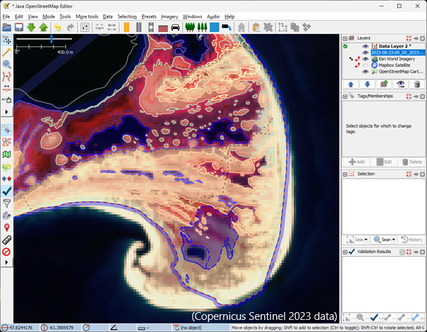Figure 8: Updated OSM data overlaid on a recent Sentinel-2 image shows differences of up to 400 meters between shoreline locations (Copernicus Sentinel 2023 data)

Bare coastal lands: These features fall into two categories. Features at sea level such as beaches or breakwaters, and features overhanging the coastline such as bare rocks, screes, and cliffs. These overhanging features often required using the Mapbox image to avoid significant distortions due to elevation changes.

Natural features: Islands’ natural landscape consists mainly of grasslands with large patches of forest and wetlands. Long beaches, sand barriers and dunes connect the islands together, creating large lagoons. So, traveling around the islands and hiking a few trails was necessary to later interpret this complex set of features (Figure 9).

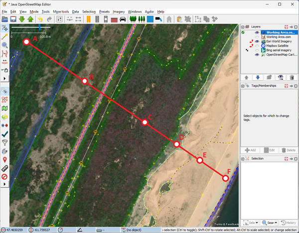Figure 9: Adjacent natural features (A-F): string bog, scattered shrubs, stunted wood, grassland, sand dunes, beach.

I identified five types of vegetation: grasslands, heather, shrubland, wetlands and woodland; Forest is mostly made up of evergreen needle leaved vegetation. Tree heights vary greatly depending on their location, ranging from normal inland to stunted trees on hilltops and near the coast. Identifying wetland types was also difficult and often like dividing shades of gray into categories. I nevertheless assigned a wetland=* tag value to all of them, including on some string bogs. However, these string bogs, as well as most inland salt marshes, were fossilized landforms (i.e., no longer active). It was the same for the sand dunes system, although I didn’t try to map the landform. While active dunes were easy to identify, it was difficult to choose whether to tag them as sand, or grasslands as the vegetation was taking over. Finally, most water bodies were already mapped and therefore only needed some adjustments to their shore and tags. Some closed (or almost closed) bodies of water were converted from “coastline” to “lagoon”.

Land use: This feature subset included both the usual landuse=* tag values as well as parking lots. Farmland is the main land use I identified, although I was only able to find a few farmyards. Next come the residential areas, then the industrial ones. The largest industrial complex on the islands is the Cap-aux-Meules thermal power plant, followed by the Seleine salt mine.

Buildings, service roads, tracks, and trails: I mapped the buildings in two iterations. I first used Mapbox for buildings’ geometry, as its near-vertical viewing angle minimized distortions. I then used Esri World to update the result since the image was more recent. In doing so, I found many buildings that had disappeared, in the meantime, especially near the coast. Browsing local newspapers, I discovered that most of them had been destroyed in severe storms over recent years. To make sure other mappers would not map them again using older images, I kept them in the database while using a life cycle prefix to turn them off on the map (Figure 10). Outside of urban areas, most family housing units consist of a detached house, a garage, and a shed. These units are generally dispersed across the landscape and connected to the road network by long driveways.

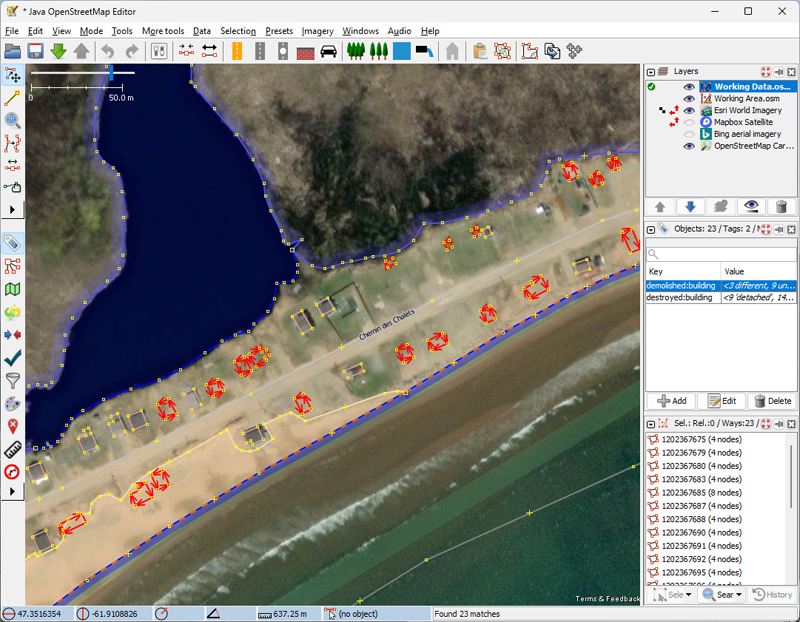Figure 10: Destroyed/demolished buildings after recent severe storms (in red). Esri World image (Îles-de-la-Madeleine).

I complete my mapping with tracks and trails, which have little topological relationship with the previous features. There is an extensive track network on the islands, most related to farming or tourism (including all-terrain vehicles). Due to islands ground characteristics, it is difficult to know whether these tracks contain compacted material or not, without going through each one. So, when in doubt, I assumed they did not (i.e., tracktype=grade5). As for the trails, it seems I was preceded by a few OSM contributors. None of the trails I walked through were missing, so I just had to adjust a few of them to fit SGH data.

Thoughts About the Project

This was my longest mapping project, and I learned a lot from mapping such a diversity of natural map features. Here are my thoughts about what went right, should be done differently, and could have helped.

What went right: Obviously, most of the mapping went right. My crush is having discovered the Strava Global Heatmap (SGH). After using OSM’s GPS tracks for years, I was blown away by the volume of tracks found in SGH, their display (i.e., data density), and ease of use in JOSM. From now on, I will continue to use SGH for all my mapping projects, both to adjust images when necessary, and to find/confirm the locations of popular hiking trails.

The next thing is to have kept track of mapped areas (via a dedicated file) and features (via iterative data capture). It really simplified my work. I could have mapped one feature at a time over all the islands, but the pleasure of seeing the map get colored, one patch at a time, motivated me to continue.

Finally, I will keep using life cycle prefixes when required. This allowed me to remove buildings from the map while keeping them in the database. Until all images tell the same story, it may prevent other mappers from capturing them again by using older images.

What should be done differently: My main concern is that in my eager to map, I have started merging identical natural features into single multipolygons, for efficiency. As all these features were going to be set as multipolygons anyway, it was faster to proceed that way than to create a new multipolygon, duplicating tags, and so on, for each individual occurrence. One could argue it all depends on what a multipolygon relation represents. An isolated feature? All the occurrences of a feature in a specific context (e.g., the wooded areas of a nature reserve)? If for some instances, I would do the same (Figure 11), I am quite sure I could not use this argument for many others.

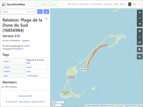Figure 11: Plage de la Dune-du-Sud (Îles-de-la-Madeleine). The beach is mapped as a 22 km long multipolygon.

As far as I know, there is no consensus within the OSM community as to the best way to map adjacent polygons. I prefer using multipolygons rather than duplicating common line segments of adjacent polygons. However, the downside of using multipolygons is that it can be more difficult for new contributors to modify them. Having multiple outer rings spread around for a feature, unless really required, can only make things worse. I’ll probably try to fix the worst cases manually over the next few months.

Another thing I should have done differently is to use Sentinel-2 imagery in a first iteration to map the coastline. I would have kept the location of the coastline and adapted my mapping using older available images in a second iteration (Figure 8). These older images are probably just fine around cliffs/rocky shores, but Sentinel-2 data should have been used where coastal dynamics is important (i.e., erosion and deposition).

What could have helped: Image metadata would make it easier to decide which image to use. Without knowing about the recent storms and seeing their impacts on the ground, I probably would have used Mapbox Satellite instead of Esri World. The same goes for the eastern end of the islands where I could not identify which was the most recent image.

What is next: I just hope to return to the Îles-de-la-Madeleine soon for another vacation!