At State of the Map US last month, I presented my latest OSM analysis work. This is work done in collaboration between the University of Colorado Boulder and Mapbox. You can watch the whole presentation here or read on for a summary followed by extra details on the methods with some code examples.

OpenStreetMap is Constantly Improving

At the root of this work is the notion that OSM is constantly growing. This makes OSM uniquely different from other comparable sources of geographic information. To this extent, static assessments of quality notions such as completeness or accuracy are limited. For a more wholistic perspective of the constantly evolving project, this work focuses on the growth of the map over time.

Intrinsic Data Quality Assessment

Intrinsic quality assessment relies only internal attributes of the target data and not on external datasets as points of reference for comparison. In contrast, extrinsic data quality assessments of projects like OSM and Wikipedia involve comparing the data directly to the external datasets, often authoritative, reference datasets. For many parts of the world, however, such datasets do not exist, making extrinsic analysis impossible.

Here we look at features of the OSM database over time. By comparing attributes like numbers of contributors, density of buildings, and amount of roads, we can learn how the map grows and ultimately improves overtime.

Specifically, we aim to explore the following:

Contributors

• How many?
• How recent?
• What type of edits?

Objects

• What types?
• How many?
• Relative Density?
• Object version?

The bulk of this work involves designing a data pipeline to better allow us to ask these types of questions of the OSM database. This next section takes a deep dive into these methods. The final section, Visualizing, has a series of gifs that show the results to-date.

The interactive version of the dashboard in these GIFS can be found here: http://mapbox.github.io/osm-analysis-dashboard

---

Methods: Vector Tiles

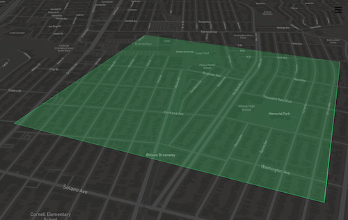
Specifically, zoom level 15 vector tiles are the base of this work. Zoom level 15 is chosen because (depending on Latitude), most tiles have an area of 1 square kilometer. For scale, a zoom 15 tile looks like this:

Vector Tiles are chosen primarily for three reasons:

1. Vector Tiles (specifically OSM data in the .mbtiles format) are standalone sqlite databases. This means very little overhead to maintain (no running database). To this end, they are very easy to transfer and move around on disk.

2. They are inherently a spatial datastore. With good compression abilities, the file sizes are not dramatically larger than standard osm pbf files, but they can be loaded onto a map with no processing. This is mostly done with mbview
3. Vector Tiles can be processed efficiently with the tile-reduce framework.

In sum, at any point in the process, a single file exists that can easily be visualized spatially.

Quarterly Historic Snapshots

To capture the growth of the map overtime, we create historical snapshots of the map: OSM-QA-Tiles that represent the map at any point in history. You can read more about OSM-QA-Tiles here.

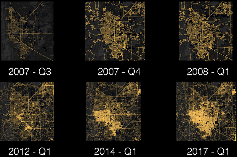
This image shows the growth of Boulder, CO in the last decade. The top row shows the road network rapidly filling in over 9 months during the TIGER import and the bottom row shows the the densification of the road and trail network along with the addition of buildings over the last 5 years.

The global-scale quarterly snapshots we created are available for download here: osmlab.github.io/osm-qa-tiles/historic.html.

While quarterly snapshots can teach us about the map at a specific point in history, they do not contain enough information to tell us how the map has changed: the edits that happen between the quarters. To really answer questions such as, “how many users edited the map?” or “How many kilometers of roads were edited?” or “How many buildings were added?” We need the full editing history of the map.

Historical Tilesets

The full editing history of the map is made available in various formats on a weekly basis. Known as the full history dump, this massive file can be processed in a variety of ways to help reconstruct the exact process of building the map.

Since OSM objects are defined by their tags, we focus on the tagging history of objects. To do this, we define a new schema for historical osm-qa-tiles. The new vector tiles extend the current osm-qa-tiles by including an additional attribute, @history.

Currently, these are built with the OSM-Wayback utility. Still in development, this utility uses rocksdb to build a historical tag index for every OSM object. It does this by parsing a full-history file and saving each individual version of each object to a large index (Note: Currently only saves objects with tags, and does not save geometries). This can be thought of as creating an expanded OSM history file that is optimized for lookups. For the full planet, this can create indexes up to 600GB in size.

Once the index is built, the utility can ingest a ‘stream’ of the latest OSM features (such as those produced by minjur or osmium-export). If the incoming object version is greater than 1, then it performs a lookup for each previous version of the object in this index.

The incoming object is then augmented to have an additional @history property. The augmented features are then re-encoded with tippecanoe to create a full-historical tileset.

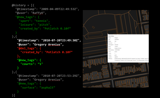
Here is an example of a tennis court that is currently at version 3 in the database. The @history property contains a list of each version with details about which tags were added or deleted in each version.

A Note on Scale & Performance

Full history tilesets are rendered at zoom level 15. OSM-QA-Tiles are typically rendered only at zoom level 12, but we found zoom 15 to be better not only for the higher resolution, but it lowers the number of features per tile. Since many features are now much larger because they contain multiple versions, this helps lower the number of features per tile, keeping tile-reduce processing efficient.

One downside, however, is that at zoom 15, the total number of tiles required to render the entire planet can be problematically large (depending on the language/library reading the file). For this reason, historical tilesets should be broken into multiple regions.

Processing 1: Create Summary Tilesets

The first step in processing these tiles is to ensure that the data are at the same resolution. Historical tilests are created at zoom 15 resolution while osm-qa-tiles exist at zoom 12 resolution. Zoom 12 is the highest resolution that the entire planet should be rendered to osm-qa-tiles to ensure efficiency in processing. Therefore, we start by summarizing zoom 15 resolution into zoom 12 tiles.

Summarizing Zoom 15 Resolution at Zoom 12

A zoom-12 tile contains 64 child zoom-15 tiles (64 tiles = 4^(15-12), resulting in an 8x8 grid). To create summary tilesets for data initially rendered at zoom 12 (like the snapshot osm-qa-tiles), we calculate statistics about each child zoom-15 tile inside of a zoom-12 tile. This is done with a tile-reduce script that first bins each feature into the appropriate 64 child zoom-15 tiles and then computes various statistics for each of them, such as “total kilometers of named highway” or “density of buildings”

Since each of these attributes pertains to the zoom-15 tile and not individual features, individual object geometries are ignored. Instead, these statistics are represented by a single feature: a point at the center of the zoom-15 tile that it represents. Each feature then looks like:

geometry: <Point Geometry representing center of zoom-15 tile>
properties : {
   quadkey :		<unique quadkey for zoom 15 tile>,
   highwayLength:		<total length of highways>,
   namedHighwayLength:	<kilometers of named highways>,
   buildingCount:			<Number of buildings>,
   buildingArea:			<Total area of building footprints>
   ...

These features are encoded into zoom-12 tiles, each with no more than 64 features. The result is a lightweight summary tileset (only point-geometries) rendered at zoom-12.

Summarizing Editing Histories

The summarization of the editing histories is very similar, except that the input tiles are already at zoom 15. Therefore, we skip the binning process and just summarize the features in each tile. Similarly, up to 64 individual features that each represent a zoom-15 tile are re-encoded into a single zoom-12 tile. Each feature includes editing statistics per-user for the zoom-15 tile it represents:

geometry: <Point Geometry representing center of zoom-15 tile>
properties : {
  quadkey : (unique quadkey for zoom 15 tile),
  users: [
  {
    name: <user name>,
    uid: <user id>,
    editCount: <total number of edits>,
    newFeatureCount: <number of edits where version=1>,
    newBuildings: <number of buildings created>,
    editedBuildings: <number of buildings edited>,
    newHighwayKM: <kilometers of highways created>,
    editedHighwayKM: <kilometers of highways edited>,
    addedHighwayNames: <Number of `name` tags added to highways>,
    modHighwayNames: <Number of existing `name` tags modified on highways>
  },
  { ... }
],
usersEver: <array of all user ids ever to edit on this tile>

Why go through all of this effort to tile it?

Keeping these data in the mbtiles format enables spatial organization of the editing summaries in a single file. Encoding zoom 15 summaries into zoom 12 tiles is the ideal size for the mbtiles format and can be efficiently processed with tile-reduce.

Processing 2: Calculate & Aggregate

With the above summarization, we have two tilesets each rendered at zoom 12 with zoom 15 level resolution. We can now pass both tilesets into a tile-reduce script. This is done by specifying multiple sources when initializing the tile-reduce job:

var tileReduce = require('@mapbox/tile-reduce');

tileReduce({
  zoom: 12,
  map: path.join(__dirname, '/map-tileset-aggregator.js'),
  sources : [{
    name: 'histories',
    mbtiles: historicalTileset-2010-Q4,
    raw: false
   },{
    name: 'quarterly-snapshot',
    mbtiles: snapshot-2010-Q4,
    raw: false
  }]
  ...

In processing, the map script can then access attributes of both tilesets like this:

module.exports = function(data, tile, writeData, done) {  
  var quarterlySnapshots = data['quarterly-snapshot']
  var histories = data['histories']

For performance, the script builds a Map() object for each layer, indexing by zoom-15 quadkey. Next, the script iterates over the (up to 64) features of one tile and looks up the corresponding quadkey in the other tile to combine, compare, contrast, or calculate new attributes. Here is an example of combining and aggregating across two tilesets, writing out single features with attributes from both input tilesets:

features.forEach(function(feat){

  //Create a single export feature to represent each z15 tile:
  var exportFeature = {
    type      : 'Feature',
    tippecanoe: {minzoom: 10, maxzoom: 12}, //Only renders this feature at these zoom levels.
    properties: {
      quadkey   : feat.properties.quadkey //The z15 quadkey
    },
    geometry: tilebelt.tileToGeoJSON(tilebelt.quadkeyToTile(feat.properties.quadkey)) // Reconstruct the Polygon representing the zoom-15 tile.
  }
  
  exportFeature.properties.buildingCount_normAggArea  =  < Lookup the number of buildings on this zoom-15 tile (and normalize by area).
  exportFeature.properties.namedHighwayLength_normAggArea = < Lookup kilometers of named highway for this zoom-15 tile (and normalize by area).
  
  // Access the contributor history information for this zoom-15 tile.
  var tileHistory  = contributorHistories.get(feat.properties.quadkey)
  var users = JSON.parse(tileHistory.users) // Get user array back from string
  
  // Sum attributes across users for simple data-driven-styling
  users.forEach(function(user){
    exportFeature.properties.editCount         += user.editCount;
    exportFeature.properties.newFeatureCount   += user.newFeatureCount;
    exportFeature.properties.newBuildings      += user.newBuildings;
    exportFeature.properties.newHighwayKM      += user.newHighwayKM;
    exportFeature.properties.editedHighwayKM   += user.editedHighwayKM;
    exportFeature.properties.addedHighwayNames += user.addedHighwayNames;
    exportFeature.properties.modHighwayNames   += user.modHighwayNames;
  });
  writeData( JSON.stringify( exportFeature ) ) //Write out zoom-15 tile summary with information combined from both tilesets.
})

This script produces two types of output:

1. (Up to 64) polygons per zoom-12 tile that represent the child zoom-15 tiles. Matching the editing-history format, these features contain per-editor statistics, such as kilometers of roads.

2. A single zoom-12 summary of all the editing activity.

Processing 3: The Reduce Phase

When the summary zoom-12 tile is delivered to the reduce script, it is first written out to a file (z12.geojson) and then passed to a downscaling, aggregation function, described next.

Downscaling & Aggregation

Last year I made a series of similar visualizations of osm-qa-tiles. I only worked with the data at zoom 12 and kept the features very simple in hopes that tippecanoe could coalesce similar features to display at lower zooms. While this worked, there were a lot of visual artifacts in busy parts of the map and the tile individual geometries must be low detail to fit:

To address this, we rely heavily on downscaling and aggregation in the current workflow to successively bin and summarize children tiles into a single parent child. Each zoom level is then written to disk separately and tiled only at specific zoom levels. Unfortunately, this is done by holding these tiles in memory. Fortunately, however, with a known quantity of (4) child tiles per parent zoom level, we can design the aggregation to continually free up memory when all child tiles of a given parent tile are processed.

Psuedocode:

zoom_11_tiles = {
   'tile1' : [],
    ...
   'tileN' : []
 }
 
processTile( incomingTile (Tile at Zoom 12) ){
  z11_parentTile = incomingTile.getParent()
  tiles_at_zoom_11[z11_parentTile].push(incomingTile)
  if (tiles_at_zoom_11[parent].length == 4){
	
    // Aggregate, Sum, Average attributes 
    // of zoom 12 tiles as appropriate to create
    // single summary zoom 11 tile
    
    // Write aggregated, summarized zoom 11 
    // tile to disk and delete from memory.
  }
}

In reality, these are not done for every zoom level, but instead for zoom levels 12, 10, and 8.

To ensure this function works as designed, the order of tiles being processed by the entire tile-reduce job is modified to be a stream of tiles grouped at zoom 10. While we cannot ensure that tiles finish processing in a specific order, by controlling the order of the input stream, we can create reasonable expectations that groups of tiles finish processing at similar times and are therefore appropriately aggregated and subsequently freed from memory.

Processing 4: Tiling

The final result of the tile-reduce job(s) is a series of geojsonl files (line-delimited) representing different zoom levels. Using tippecanoe, we create a single tileset that is optimized for rendering in the browser. Recall that each geometry is a polygon representing a vector tile. The attributes of each feature are consistent among zoom levels to allow for data-driven styling in mapbox-gl.

tippecanoe -Z0 -z12 -Pf --no-duplication -b0 \
  --named-layer=z15:z15-res.geojsonl \
  --named-layer=z12:z12-res.geojsonl \
  --named-layer=z10:z10-res.geojsonl \
  --named-layer=z8:z8-res.geojsonl   \
  -o Output.mbtiles

Visualizing: Mapbox-GL

Loading the resulting tileset into MapboxGL allows for data driven styling across any of the calculated attributes. An interactive dashboard to explore the North America Tileset is available here: mapbox.github.io/osm-analysis-dashboard

Downscaling across Zoom Levels

This first gif shows the different layers (the results of the downscale & aggregation):

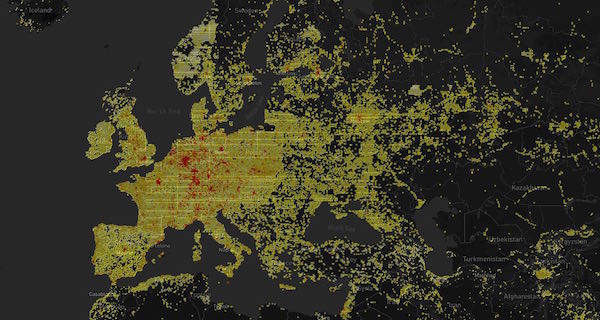
Since everything is aggregated per-quarter, we can easily compare between two quarters. This gif compares the number of active users in mid 2012 to mid 2017.

New Building Activity

Here is a high level overview of where buildings were being added to the map in the second quarter of both 2015 (left) and 2016 (right). We can see a few major building imports taking place between these times as well as more general coverage of the map.

If we zoom in on Los Angeles and visualize the “building density” as calculated in July 2015 and July 2016, we see the impact of LA building import at zoom 15 resolution:

Users

The 2010 Haiti Earthquake:

This slider shows the number users active in Haiti during the last quarter of 2009 (just before the earthquake) and then the first quarter of 2010 (when the earthquake struck):

We can see the work done by comparing the building density of the map at the end of 2009 and then at the end of the first quarter of 2010:

Ultimately, the number of (distinct) contributors active to date in North America has grown impressively in the last 5 years. This animation shows the difference between mid 2012 and mid 2017:

Looking Forward: Geometric Histories

So far, when discussing full editing history, we’ve only been talking about history of a map object as told through the changes to tags over time. This is a decent proxy of the total editing, and can certainly help us understand how objects grow and change overtime. The geometries of these objects, however also change overtime. Whether it’s the release of better satellite imagery that prompts a contributor to re-align or enhance a feature, or just generally squaring up building outlines, a big part of editing OpenStreetMap includes changing existing geometries.

Many times, geometry changes to objects like roads or buildings do not propagate to the feature itself. That is, if only the nodes underlying a way are changed, the version of the way is not incremented. Learning that an object has had a geometry change requires a more involved approach, something we are currently exploring in addition to just the tag history.

With full geometry history, we could compare individual objects at two points in time. Here is an example from a proof-of-concept for historic geometries. Note many of the buildings initially in red “square up” when they turn turquoise. These are geometry changes after the 2015 Nepal Earthquake. The buildings were initially created non-square and just a little while later, another mapper came through and updated the geometries: